Detailed control sequence of RISC-V with timing diagram https://youtu.be/4Sal1Goe2WE
RISC-V simulator with controls. (including demo) https://youtu.be/YI43OAhvTOw
How to add a new instruction to RIS-V simulator https://youtu.be/YoYxkNfTs9g
(Python code main.py.txt rv32c.py.txt load32.py.txt zip-all)
The goal of this project is to create a detailed control sequences of RISC-V to compliment the explanation in the book by D. Patterson, J. Hennessy, "Computer Organization and Design: The hardware/software interface (RISC-V edition)," Morgan Kaufman, 2018. The purpose of this interpreter is for teaching a class in computer architecture for engineering students.
With this simulator, students can see the timeline of the control events (assertion of control signals) in details and should have a better idea of how the control unit of a version of RISC-V works. Experiment with creating "special" instruction is not difficult. Students can modify the source code (written in Python) to create different sequences to achieve the desired effect.
The simulator is created according to the design of RISC-V explained in the textbook. The following diagram is similar to the standard one in the book with additional "naming" of wires and ports for wires and registers in the simulator.
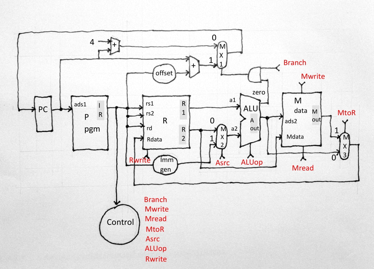
<Figure 1 Diagram of RISC-V datapath and control names, control signals in red>
Here is the overall picture of the control unit behaviour. It implements only 9 basic instructions with 32-bit data width. The control signals in the textbook is in red. The internal registers (internal) are used to hold the value in the simulator when they connect to output wires. These wires are used as inputs for other functional units.

<Figure 2 RISC-V Control signals timing diagram. It shows the "sequence" of actions. The timeline is not to scale. It is drawn corresponded to the width of datapath above (Fig.1). The actual length of time depends on the circuit design.>
The "structure" part of the simulator consists of functional units corresponded to datapath. There are Program Counter (PC), Instruction memory (P), Registers (R), ALU, and Data memory (M) with three multiplexors: mx1, mx2, mx3. The decoding of an instruction is a bit complex. They are represented by the units: Immediate generator (Imm gen) and Offset (decode the value of offset of branch instructions). Each functional units are described in details below. The control signals are denoted by <sig> which is orchestrated by the Control. Control is the "behavioural" part of the simulator. We will explain more in the next section.
functional units are: PC, P, R, ALU, M
multiplexor: mx1, mx2, mx3
PC program counter
input: next PC
output: PC
control: read and update (implicit)
P instruction memory
input: ads1
internal: IR (keep current instruction)
output: IR
control: read P (implicit)
R registers
input: rs1, rs2, rd, Rdata
internal: R1,R2,
output: R1,R2
control: <Rwrite>
ALU
input: a1, a2
internal: Aout
out: Aout, zero
control: <ALUop>
M data memory
input: ads2
internal: Mout
output: Mout
control: <Mread>,<Mwrite>
multiplexor
mx1 select next PC
input0: PC+4
input1: PC+offset
control: <branch> and zero
mx2 select input a2 to ALU
input0: R2
input1: imm
control: <Asrc>
mx3 select data to write back to R
input0: Aout
input1: Mout
control: <MtoR>
The "behavioural" part of the simulator determined the sequences of data flow between functional units to achieve the result of executing an instruction. The control is modeled after the explanation of RISC-V in the textbook. Some design decision how datapath should behaved is made by me (the author of this simulator).
A complete instruction execute cycle consists of five stage: fetch,
decode, execute, memory, writeback. The first two stages, fetch and
decode, are the same for all instructions. The remaining three
stages performed differently for different instructions. The toplevel
execution cycle is as follows.
PC = 0

          while (not stop)

               fetch

               decode

               execute

               memory

               writeback
a -> b. The a -> b;c
denotes b and c occurs simultaneously.fetch
get a word from P memory -> IR
decode
IR -> op,rd,rs1,r2, compute imm, offset
imm -> mx2_1
offset+PC-> mx1_1
select control-vector
The last three stages use control-vector to represent the different actions of different instruction. Decode stage selects the appropriate control-vector that is used in the last three stages. Control signals are explained in the next section. zero is an output from ALU which is the result of ALU operations. Its value is boolean True/False. It is used in conjunction with <Branch> control signal to determine the next PC (next instruction or branch to target address).
execute

              read R

              R[rs1] -> R1-> a1

              R[rs2] -> R2->mx2_0;Mdata


              <Asrc> mx2 ->a2

              <ALUop> ->Aout->ads2;mx3_0

              <branch> mx1

                   if zero


          PC+mx1_1->PC  (branch taken)

                   else


          PC+mx1_0->PC  (next)
memory

              <Mread>  M[ads2] -> Mout->mx3_1

              <Mwrite> Mdata->M[ads2]
writeback <MtoR> mx3->R[Rdata] <Rwrite>
Control-vector represents a group of control sequence for each
instruction. The control signals are of two types, one type is for
multiplexor (0/1 select port 0/1) , the other type is active/not-active
(1/0) such as <Mread>. The only exception is the <ALUop> which
denotes functions of ALU (currently implement only: add, sub, eq, ne, lt,
ge). The control signals are ordered by time from left to right.
[
          <Asrc>,<ALUop>,<branch>,<Mread>,<Mwrite>,<MtoR>,<Rwrite>
          ]
Asrc: {0,1} mx2
ALUop: {0,1,2,3,4,5,6,7} 0and, 1or, 2add, 3sub, 4eq, 5ne, 6lt,
7ge
branch: {0,1} mx1
Mread: {0,1} 1 - active
Mwrite: {0,1} 1 - active
MtoR: {0,1} mx3
Rwrite: {0,1} 1 - active
Here is the control-vector of each instruction.
[
          <Asrc>,<ALUop>,<branch>,<Mread>,<Mwrite>,<MtoR>,<Rwrite>
          ]


          add:  [0,2,0,0,0,0,1]

          sub:  [0,3,0,0,0,0,1]

          addi: [1,2,0,0,0,0,1]

          lw:   [1,2,0,1,0,1,1]

          sw:   [1,2,0,0,1,1,0]

          beq:  [0,4,1,0,0,0,0]

          bne:  [0,5,1,0,0,0,0]

          blt:  [0,6,1,0,0,0,0]

          bge:  [0,7,1,0,0,0,0]
Let us use "add x2,x3,x4" to show a detailed execution of
datapath according to our simulator.
fetch: the instruction is read from P[PC]. Let the value be stored in IR.
decode: various values are extract from fields in IR to become rd, rs1, rs2. Offset and Imm gen also output the appropriate values (for this instruction, they are not used). The control-vector [0,2,0,0,0,0,1] is selected.
execute: Two registers indexed by rs1 and rs2 are read and store to R1, R2. Control signals from the control-vector are asserted.
<Arc> select port 0, value of R2 is fed to a2 of ALU.memory: it is not load/store instruction.
<Mread> 0 not activewriteback:
<MtoR> 0 select Aout to write back to registerThe control sequence of other instruction can be similar explained.
The simulator is written in Python. There are three files. main.py contains user command line interface. rv32c.py is the datapath and control simulation. load32.py contains supporting functions such as loading the object file, encode and decode, disassemble the instructions.
The simulator implements 9 instructions: add, addi, lw, sw, beq, bne, blt, bge. The datawidth is 32-bit. The instruction and data memory are unified. There are 1000 words of memory (because of lw/sw, addressing on word boundary). The simulator stops when encounter "nop" (op = 0) instruction or executing more than MAXRUN (10000 cycles).
The input object code file to the simulator is the text file, each line contains a 8-digit hexadecimal number coding a machine instruction. The rest of a line is ignored so it can be used to keep the assembly code. Here is an example of a program to add 1 to 5 result in x4. The assembly code is assembled with Venus (RISC-V online interpreter) https://venus.cs61c.org/
0x00000213  addi x4 x0 0

        0x00100293  addi x5 x0 1

        0x00500313  addi x6 x0 5

        0x00534863  blt x6 x5 16

        0x00520233  add x4 x4 x5

        0x00128293  addi x5 x5 1

        0xFE000AE3  beq x0 x0 -12
Starting by activating "main.py", assume we run with a console. Here is what shows on the screen. We load the above object file named "add1-5.obj" into the simulator. "t" runs one step (one instruction). "g" runs until the program ends (hits "nop" instruction). The output shows the control-vector, next pc, the current instruction and the state of registers after executing the current instruction. Type "h" will show you more available commands including command to set memory, show range of memory, and show all registers.
>>> %Run main.py

        object file:add1-5.obj

        load program, last address  7

        >t

        [1, 2, 0, 0, 0, 0, 1]

        next pc  4

        pc 0  addi x4 x0 0   x1:0 x2:0 x3:0 x4:0 x5:0 x6:0 x7:0
        x8:0 x9:0 x10:0

        >t

        [1, 2, 0, 0, 0, 0, 1]

        next pc  8

        pc 4  addi x5 x0 1   x1:0 x2:0 x3:0 x4:0 x5:1 x6:0 x7:0
        x8:0 x9:0 x10:0

        >g

        [1, 2, 0, 0, 0, 0, 1]

        next pc  12

        pc 8  addi x6 x0 5   x1:0 x2:0 x3:0 x4:0 x5:1 x6:5 x7:0
        x8:0 x9:0 x10:0

        ....

        pc 24  beq x0 x0 -12   x1:0 x2:0 x3:0 x4:15 x5:6 x6:5
        x7:0 x8:0 x9:0 x10:0

        [0, 6, 1, 0, 0, 0, 0]

        branch taken

        next pc  28

        pc 12  blt x6 x5 16   x1:0 x2:0 x3:0 x4:15 x5:6 x6:5 x7:0
        x8:0 x9:0 x10:0

        [0, 0, 0, 0, 0, 0, 0]

        next pc  32

        pc 28  nop    x1:0 x2:0 x3:0 x4:15 x5:6 x6:5 x7:0
        x8:0 x9:0 x10:0

        >q

        >>>
Let me emphasized here again that the purpose of this simulator is not for practicing RISC-V assembly programming as this simulator implements only tiny number of instructions. There are many excellent online interpreters for that purpose (Venus is one of them). I hope that this simulator shows detailed sequences of step-by-step execution cycle of RISC-V as explained in the textbook (a few bit of details are filled in by me). The result of running these few instructions just show us that this control sequence is indeed correct. You can fully understand the working of control sequence by studying the main part of the simulator. It is less than 100 lines of code. You can also do some exercise of "creating" a control sequence for additional instruction by modifying the simulator. Have fun !!!
last update 28 Feb 2022